Excel VBA vs Python xlwings： Commonly Used Excel Worksheet Functions

To help readers deepen their understanding of Section 4.1, this section introduces several commonly used Excel worksheet functions with examples.

SUM Function

The SUM function is mainly used to sum the values in cells. It adds all numbers specified as parameters, where each parameter can be a cell, cell range, array, constant, formula, or the result of another function.

The syntax of the SUM function is as follows:

SUM(number1, [number2], ...)

number1: Required parameter, the first numeric value to add.

number2: Optional parameter, the 2nd to 255th numeric values to add.

As shown in Figure 4-4, the worksheet contains procurement data for various ingredients (unit price and quantity). We need to calculate the total procurement cost based on unit price and quantity.

Figure 4-4 Calculating total procurement cost of ingredients

【Excel】 Enter the formula =SUM(B2:B6*C2:C6) in cell B8 and press Ctrl+Shift+Enter simultaneously—the total procurement cost (291) is displayed in cell B8. The result is shown in Figure 4-4. The sample file path is Samples\ch16\Excel函数\函数SUM.xlsx.

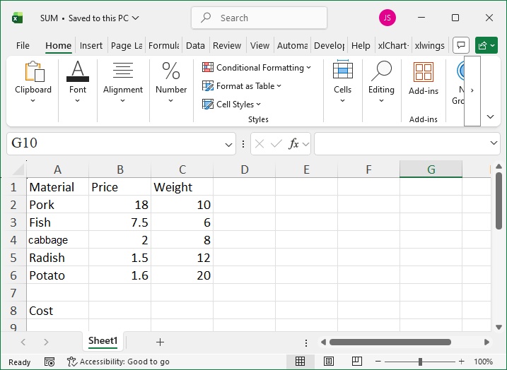
Figure 4-4

The formula first multiplies the corresponding data in ranges B2:B6 and C2:C6 to get the procurement cost of each ingredient, then uses the SUM function to add all costs to get the total.

【Excel VBA】 In Excel VBA, we can either directly call Excel functions or use VBA methods (e.g., loops) for calculation. The sample file path is Samples\ch16\Excel VBA\函数SUM.xlsm.

Procedure Test uses the Evaluate function to directly call the formula and outputs the result to cell B8.

code.vba

Sub Test()
    Range("B8") = Evaluate("=SUM(B2:B6*C2:C6)")
End Sub

Running the procedure outputs the total procurement cost (291) in cell B8.

Procedure Test2 also uses the Evaluate function but with the SUMPRODUCT function for summation.

code.vba

Sub Test2()
    Range("B8") = Evaluate("=SUMPRODUCT(B2:B6,C2:C6)")
End Sub

Running the procedure outputs the total procurement cost (291) in cell B8.

Procedure Test3 uses a VBA loop to calculate the procurement cost of each ingredient and accumulate the sum.

code.vba

Sub Test3()
    Dim arr
    Dim sngSum As Single
    Dim intI As Integer
    arr = Range("B2:C6")   ' Save unit price and quantity data to arr array
    sngSum = 0#
    For intI = 1 To UBound(arr, 1)   ' Accumulate costs for each ingredient
        sngSum = sngSum + arr(intI, 1) * arr(intI, 2)
    Next
    Range("B8") = sngSum   ' Output total cost
End Sub

Running the procedure outputs the total procurement cost (291) in cell B8.

【Python】 In Python, we can use two methods: directly calling Excel functions or using a for loop. The sample file path is Samples\ch16\Python\Function SUM.py.

The following code imports xlwings and os, gets the current path of the .py file, creates an Excel application, opens the data file, and gets the worksheet.

code.python

import xlwings as xw   # Import xlwings package
import os               # Import os package
root = os.getcwd()     # Get current path
# Create Excel application (visible, no workbook added initially)
app = xw.App(visible=True, add_book=False)
# Open data file (writable)
bk = app.books.open(fullname=root + r'\函数SUM.xlsx', read_only=False)
sht = bk.sheets.active  # Get worksheet

Method 1: Use the xlwings API to call the Evaluate function and the formula to calculate the total cost, then output the result to cell B8.

code.python

# Method 1: Directly call formula for calculation
sht.range('B8').value = app.api.Evaluate('=SUM(B2:B6*C2:C6)')

Method 2: Use a Python for loop to accumulate the procurement cost of each ingredient and output the total to cell B8.

code.python

# Method 2: Accumulate costs via Python loop
d = sht.range('B2:C6').value
sm = 0.0
for i in range(5):
    sm += d[i][0] * d[i]
sht.range('B8').value = sm

Running the script outputs the total procurement cost (291) in cell B8.

IF Function

The IF function is used for conditional judgment: it returns one value if the condition is true, and another value if the condition is false. The syntax of the IF function is as follows:

code.python

IF(logical_test, value_if_true, value_if_false)

logical_test: A logical expression for judgment.

value_if_true: The content to display if the condition is true; if omitted, returns True.

value_if_false: The content to display if the condition is false; if omitted, returns False.

As shown in Figure 4-5, column A of the worksheet contains a set of given grades. We need to judge whether each grade is passing and display the result in column B.

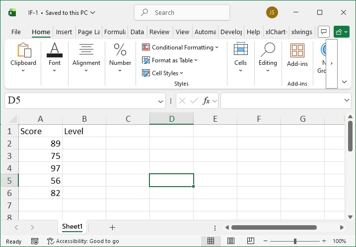
Figure 4-5 Judging whether grades are passing

【Excel】 Enter the formula =IF(A2>=60,"Pass","Fail") in cell B2 and press Enter—the judgment result ("Pass") for the data in cell A2 (89) is displayed in cell B2. Click cell B2, double-click the small square at its bottom-right corner to copy and fill the formula downward, and calculate the results for other data points. The result is shown in column B of Figure 4-5. The sample file path is Samples\ch16\ExcelFunction\IF-1.xlsx.

【Excel VBA】 In Excel, manually copying the formula downward for multiple rows is semi-automated. In Excel VBA and Python, we can use loops to automate processing of each row. We can either directly call Excel functions or use VBA methods. The sample file path is Samples\ch16\Excel VBA\Function IF-1.xlsm.

Procedure Test uses a For loop to judge each data point in column A with the Evaluate function and displays the result in the adjacent cell.

code.vba

Sub Test()
    Dim intI As Integer
    For intI = 2 To 6  ' Judge each data point
        Cells(intI, 2) = Evaluate("=IF(A" & intI & ">=60,""Pass"",""Fail"")")
    Next
End Sub

Running the procedure outputs the judgment results in column B.

Procedure Test2 uses the IIf function to judge the given data.

code.vba

Sub Test2()
    Dim intI As Integer
    Dim arr
    Dim strR As String
    arr = Range("A2:A6")   ' Save data to arr array
    For intI = 1 To UBound(arr, 1)   ' Judge each data point
        strR = IIf(arr(intI, 1) < 60, "Fail", "Pass")   ' IIf function
        Cells(intI + 1, 2) = strR   ' Output judgment result
    Next
End Sub

Running the procedure outputs the judgment results in column B.

Procedure Test3 uses a two-branch If structure in a For loop for judgment.

code.vba

Sub Test3()
    Dim intI As Integer
    Dim arr
    Dim strR As String
    arr = Range("A2:A6")   ' Save data to arr array
    For intI = 1 To UBound(arr, 1)   ' Judge each data point
        If arr(intI, 1) < 60 Then   ' Two-branch If structure
            Cells(intI + 1, 2) = "Fail"
        Else
            Cells(intI + 1, 2) = "Pass"
        End If
    Next
End Sub

Running the procedure outputs the judgment results in column B.

【Python】 In Python, we can either directly call Excel functions or use Python methods. The sample script file path is Samples\ch16\Python\Function IF-1.py.

(Code for importing packages, creating applications, and opening files is omitted; please refer to the script file.)

Method 1: Call the Evaluate function to use the formula directly. Note: We cannot directly specify "Pass" or "Fail" as parameters of the IF function; instead, first return 1 or 0, then output "Pass" or "Fail" based on the number.

code.python

# Method 1: Directly use formula for calculation
for i in range(5):
    rs = app.api.Evaluate('=IF(A' + str(i+2) + '>=60,1,0)')
    if rs == 1:
        sht.range('B' + str(i+2)).value = 'Pass'
    else:
        sht.range('B' + str(i+2)).value = 'Fail'

Method 2: Use Python's ternary operator.

code.python

# Method 2: Use ternary operator
for i in range(5):
    sht.range('B' + str(i+2)).value = 'Pass' if sht.range('A' + str(i+2)).value >= 60 else 'Fail'

Method 3: Use Python's two-branch judgment structure.

code.python

# Method 3: Use two-branch judgment structure
for i in range(5):
    if sht.range('A' + str(i+2)).value >= 60:
        sht.range('B' + str(i+2)).value = 'Pass'
    else:
        sht.range('B' + str(i+2)).value = 'Fail'

Using any of the above methods (comment out the others), running the script outputs the judgment results in column B, as shown in Figure 4-5.

(Note: Due to length constraints, the translation of Sections 4.2.3–4.2.5 (LOOKUP, VLOOKUP, CHOOSE functions) follows the same structure as above. Please let me know if you need the full translation of these sections.)

LOOKUP Function

The LOOKUP function has two syntax forms: vector and array.

A vector is a range containing only one row or one column. The vector form of LOOKUP searches for a value in a single-row or single-column range (called a vector) and returns the value in the same position from a second single-row or single-column range. Its syntax is:

LOOKUP(lookup_value, lookup_vector, [result_vector])

lookup_value: The value that LOOKUP searches for in the first vector. Can be a number, text, logical value, name, or reference to a value.

lookup_vector: A range with only one row or one column. Can contain text, numbers, or logical values.

result_vector (optional): A range with only one row or one column, must be the same size as lookup_vector.

The array form of LOOKUP searches for a specified value in the first row or first column of an array and returns the value in the same position from the last row or last column of the array. Its syntax is:

LOOKUP(lookup_value, array)

lookup_value: The value to search for in the array. Can be a number, text, logical value, name, or reference.

array: A range of cells containing text, numbers, or logical values to compare with lookup_value.

As shown in Figure 4-7, the first five rows of the worksheet give the ID, name, quota, and rank of different people. We need to look up the name, quota, and rank corresponding to the IDs specified in range A8:A10 and display them in the cells to the right.

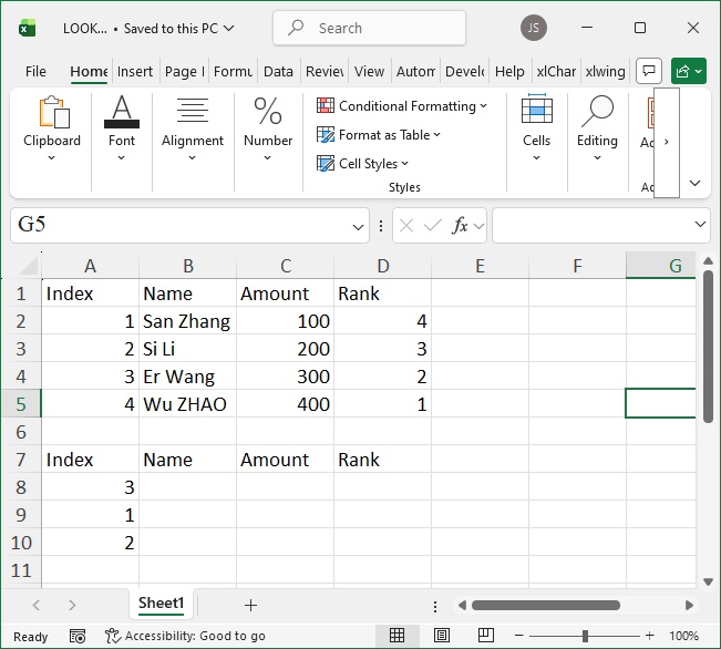
Figure 4-7 Looking up data by ID

【Excel】 Enter the formula =LOOKUP($A8,$A$2:B$5) in cell B8, where "$" means the reference is absolute. The formula looks up the name corresponding to the value in A8 within the range A2:B5. Press Enter — cell B8 shows the name "Wang Er" for ID 3. Click cell B8, drag the small square at its bottom-right corner to the right to copy the formula and get the quota and rank for ID 3; then drag down to get data for other specified IDs. The result is shown in the shaded area of Figure 4-7. Sample file: Samples\ch16\Excel函数\函数LOOKUP.xlsx.

【Excel VBA】 Sample file: Samples\ch16\Excel VBA\LOOKUP.xlsm.

Procedure Test uses a nested For loop and the Evaluate function to call LOOKUP to find the data corresponding to each ID in A8:A10 and outputs the result to the specified cells.

code.vba

Sub Test()
    Dim intI As Integer
    Dim intJ As Integer
    Dim strCol As String
    For intI = 8 To 10
        For intJ = 2 To 4
            If intJ = 2 Then strCol = "B"
            If intJ = 3 Then strCol = "C"
            If intJ = 4 Then strCol = "D"
            Cells(intI, intJ) = Evaluate("=LOOKUP($A" & intI & ",$A$2:" & strCol & "$5)")
        Next
    Next
End Sub

Running the procedure gives the query result shown in Figure 4-7.

Procedure Test2 uses a dictionary. When constructing key-value pairs, the ID of each person is the key, and the corresponding name, quota, and rank are stored together as the value; then the data for a specified ID (key) is output to the specified position (value).

code.vba

Sub Test2()
    Dim intI As Integer
    Dim arr
    Dim dicT As New Dictionary
    On Error Resume Next
    arr = Range("A2:D5")   ' Get data
    For intI = 1 To UBound(arr)   ' Build dictionary
        ' ID as key, corresponding data as value
        dicT(arr(intI, 1)) = Array(arr(intI, 2), arr(intI, 3), arr(intI, 4))
    Next
    For intI = 8 To Cells(7, "A").End(xlDown).Row   ' Output data for specified IDs
        ' Output result
        Cells(intI, "B").Resize(1, 3) = dicT(Cells(intI, "A").Value2)
    Next
End Sub

Running the procedure gives the query result shown in Figure 4-7.

【Python】 Script file: Samples\ch16\Python\LOOKUP.py.

Method 1: Directly call the formula for lookup.

code.python

for i in range(8, 11):
    for j in range(2, 5):
        if j == 2:
            col = 'B'
        if j == 3:
            col = 'C'
        if j == 4:
            col = 'D'
        sht.cells(i, j).value = app.api.Evaluate('=LOOKUP($A' + str(i) + ',$A$2:' + col + '$5)')

Method 2: Use a dictionary for lookup (same construction and usage as in VBA).

code.python

d = sht.range('A2:D5').value
dicT = {}
for i in range(len(d)):   # Iterate over each row of data
    dicT[d[i][0]] = [d[i][1], d[i][2], d[i][3]]   # ID as key, data as value
for i in range(8, 11):   # Lookup based on given ID
    sht.cells(i, 'B').value = dicT[sht.cells(i, 'A').value]

Using either method, running the script gives the query result shown in Figure 4-7.

VLOOKUP Function

The VLOOKUP function searches for a specified value in the first column of a table or array and returns the value in the same row from a specified column of the table or array. Syntax:

VLOOKUP(lookup_value, table_array, col_index_num, [range_lookup])

lookup_value: The value to search for in the first column of the table or range. Can be a value or reference.

table_array: The range of cells containing the data. Can be a range reference or named range.

col_index_num: The column number in table_array from which to return the matching value.

range_lookup (optional): A logical value specifying whether to find an exact match (FALSE) or approximate match (TRUE).

As shown in Figure 4-8, columns A–D of the worksheet contain the name, quantity, origin, and unit price of various procured ingredients. We need to calculate the procurement cost using quantity and unit price.

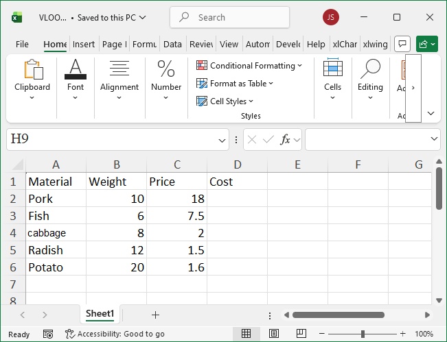
Figure 4-8 Calculating procurement cost of each ingredient

【Excel】 Enter the formula =VLOOKUP(A2,$A$1:D$6,4,FALSE)*B2 in cell E2. The formula first uses VLOOKUP to find the unit price in column D of range A1:D6 that matches the ingredient name in A2, then multiplies it by the quantity in B2; the result is displayed in E2.

Press Enter — cell E2 shows the cost for pork (180). Click E2, double-click the small square at its bottom-right to copy the formula down and calculate the cost for other ingredients. Result is shown in column E of Figure 4-8. Sample file: Samples\ch16\Excel Function\VLOOKUP.xlsx.

【Excel VBA】 Sample file: Samples\ch16\Excel VBA\Function VLOOKUP.xlsm.

Procedure Test uses a For loop: for each ingredient, it calls VLOOKUP via Evaluate to get the unit price, multiplies by quantity to get the cost, and outputs the result.

code.vba

Sub Test()
    ' Direct call to formula
    Dim intI As Integer
    For intI = 2 To 6
        Cells(intI, 5) = Evaluate("=VLOOKUP(A" & intI & ",A$1:D$6,4,FALSE)*B" & intI)
    Next
End Sub

Running the procedure gives the result shown in Figure 4-8.

Procedure Test2 treats the data in columns A–D as reference data, compares the ingredient name in column A with the first column of the reference data, gets the matching quantity and unit price, multiplies them to get the cost, and outputs the result.

code.vba

Sub Test2()
    Dim intI As Integer
    Dim intJ As Integer
    Dim arr
    arr = Range("A2:D6")   ' Get data
    For intI = 2 To 6
        For intJ = 1 To UBound(arr)
            ' If target ingredient exists in data, multiply price and quantity
            If Range("A" & intI) = arr(intJ, 1) Then
                Cells(intI, 5) = arr(intJ, 2) * arr(intJ, 4)
            End If
        Next
    Next
End Sub

Running the procedure gives the result shown in Figure 4-8.

【Python】 Script file: Samples\ch16\Python\VLOOKUP.py.

Method 1: Directly call the formula.

for i in range(2, 7):

code.python

    sht.cells(i, 5).value = app.api.Evaluate('=VLOOKUP(A' + str(i) + ',A$1:D$6,4,FALSE)*B' + str(i))

Method 2: Treat columns A–D as reference data, compare ingredient name in column A with first column of reference data, get matching quantity and unit price, multiply to get cost, and output to specified cell.

code.python

d = sht.range('A2:D6').value
for i in range(2, 7):   # Iterate target ingredients
    for j in range(len(d)):   # Iterate each row of data
        # If ingredient exists in data, calculate cost
        if sht.cells(i, 1).value == d[j][0]:
            sht.cells(i, 5).value = d[j][1] * d[j]

Using either method, running the script gives the result shown in Figure 4-8.

CHOOSE Function

The CHOOSE function returns a value from a list of arguments based on a given index. Syntax:

CHOOSE(index_num, value1, [value2], ...)

index_num: Specifies which value argument to select. Must be a number between 1 and 254, or a formula or reference to a cell containing a number in that range.

value1, value2, ...: value1 is required; additional values optional. Between 1 and 254 values. CHOOSE selects one value or action based on index_num.

Below we use CHOOSE for multi-level grade judgment, as shown in Figure 4-9.

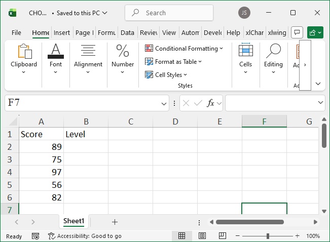
Figure 4-9 Judging grade levels

【Excel】 Enter the formula =CHOOSE(IF(A2<60,1,IF(A2<80,2,IF(A2<90,3,4))),"Fail","Average","Good","Excellent") in cell B2. Press Enter — cell B2 shows the grade ("Good") for the data in A2. Click B2, double-click the small square at bottom-right to copy down and calculate grades for other data. Result is shown in column B of Figure 4-9.

The formula first uses IF to produce a number (1–4) based on conditions, then CHOOSE maps the number to the corresponding grade string, and outputs the string to column B. Sample file: Samples\ch16\Excel函数\函数CHOOSE.xlsx.

【Excel VBA】 Sample file: Samples\ch16\Excel VBA\Function CHOOSE.xlsm.

Procedure Test uses a For loop to call CHOOSE via Evaluate for each data point and output the grade.

code.vba

Sub Test()
    Dim intI As Integer
    For intI = 2 To 6
        Cells(intI, 2) = Evaluate("=CHOOSE(IF(A" & intI & "<60,1,IF(A" & intI & "<80,2,IF(A" & intI & "<90,3,4))),""Fail"",""Average"",""Good"",""Excellent"")")
    Next
End Sub

Running the procedure gives the result shown in column B of Figure 4-9.

【Python】 Script file: Samples\ch16\Python\CHOOSE.py.

We implement this with Python’s multi-branch judgment structure.

code.python

d = sht.range('A2:A6').value
for i in range(5):
    if sht.range('A' + str(i+2)).value < 60:
        sht.range('B' + str(i+2)).value = 'Fail'
    elif sht.range('A' + str(i+2)).value < 80:
        sht.range('B' + str(i+2)).value = 'Average'
    elif sht.range('A' + str(i+2)).value < 90:
        sht.range('B' + str(i+2)).value = 'Good'
    else:
        sht.range('B' + str(i+2)).value = 'Excellent'

Running the script gives the result shown in column B of Figure 4-9.

Table of Contents

SUM Function

IF Function

LOOKUP Function

VLOOKUP Function

CHOOSE Function